Twitter Sentiment Analysis using Machine Learning on Python
₹6,000.00 Exc Tax
Twitter Sentiment Analysis using Machine Learning Algorithms on Python
Platform : Python
Delivery Duration : 3-4 working Days
100 in stock
Description
ABSTRACT
Twitter is a popular social networking website where users posts and interact with messages known as “tweets”. This serves as a mean for individuals to express their thoughts or feelings about different subjects. Various different parties such as consumers and marketers have done sentiment analysis on such tweets to gather insights into products or to conduct market analysis. Furthermore, with the recent advancements in machine learning algorithms,the accuracy of our sentiment analysis predictions is able to improve
In this report, we will attempt to conduct sentiment analysis on “tweets” using various different machine learning algorithms. We attempt to classify the polarity of the tweet where it is either positive or negative. If the tweet has both positive and negative elements, the more dominant sentiment should be picked as the final label. We use the dataset from Kaggle which was crawled and labelled positive/negative. The data provided comes with emoticons, usernames and hashtags which are required to be processed and converted into a standard form. It also need to extract useful features from the text such unigrams and bigrams which is a form of representation of the “tweet”. We use various machine learning algorithms to conduct sentiment analysis using the extracted features. However, just relying on individual models did not give a high accuracy so we pick the top few models to generate a model.
INTRODUCTION
With the huge amount of increase in the web technologies, the no of people expressing their views and the opinion via web are increasing. This information is useful for everyone like businesses, governments and individuals . with 500+ million tweets per day , twitter is becoming a major source of information. Twitter is a microblogging site, which is popularly known for its short messages known as tweets. It has a limit of 140 characters. Twitter has a user base of 240+ million active users and hence it is a useful source of information. The users often discuss their personal views on various subjects and also on current affairs via tweets. Out of all popular social medias like Facebook , Twitter, Google+, and Myspace we choose Twitter because of the reasons like
- Twitter contains vast number of text posts and it grows day by day. The collected corpus can be arbitrarily large.
- Twitter’s audience varies from regular users to celebrities, Politicians , company representatives, and even country’s president. Therefore it is possible to collect text posts of users from different social and interests groups.
- Tweets are small in length and thus less ambiguous and are unbiased in nature.
Using social media, models are built for classifying “tweets” into positive , negative, and neutral classes .The models are build for two classification tasks : a 3-way classification of already separated phrases in a tweet into positive, negative , and neutral classes and another 3 way classifications of entire message into positive , negative and neutral classes.
This paper is experimented with baseline model and feature based model. An incremental analysis is done to the features. It is also experimented with a combination of models: combining baseline and feature based model. The baseline model is done to the phrase based classification task which achieves an accuracy of 62.24% and is 29% more than the chance baseline. The feature based model uses features and achieves an accuracy of 77.86%.
These combinations achieves an accuracy of 77.90% which outperforms the baseline by 16%. For message based classification task the baseline model comes out with 51% of accuracy which is 18% more than the chance baseline. The feature based model uses the features with the accuracy of 57.43% . The combination achieves 58.00% of accuracy which outperforms the baseline by 7%.
REQUIREMENTS
Software: Anaconda – Jupyter.
Language: Python3
Modules Used:
- pickle
- nltk
- collections
- keras.models import Sequential, load_model
- keras.layers import Dense
- numpy
- sklearn.tree import DecisionTreeClassifier
- scipy.sparse import lil_matrix
- sklearn.naive_bayes import MultinomialNB
- sklearn.ensemble import RandomForestClassifier
- sklearn.feature_extraction.text import TfidfTransformer
- keras.models import Sequential, load_model
DATASET DESCRIPTION
The data given is in the form of a comma-separated values files with tweets and their corresponding sentiments. The training dataset is a csv file of type tweet_id,sentiment,tweet where the tweet_id is a unique integer identifying the tweet, sentiment is either 1 (positive) or 0 (negative), and tweet is the tweet enclosed in “”. Similarly, the test dataset is a csv file of type tweet_id,tweet.
Table1: Statistics of pre-processed train dataset
Table 2: Statistics of pre-processed test dataset
The dataset is a mixture of words, emoticons, symbols, URLs and references to people. Words and emoticons contribute to predicting the sentiment, but URLs and references to people don’t. Therefore , URLs and references can be ignored. The words are also a mixture of misspelled words, extra punctuations, and words with many repeated letters. The tweets, therefore, have to be pre-processed to standardize the dataset.
PROPOSED METHOD AND IMPLEMENTATIONS
Pre-Processing
Raw tweets scraped from twitter generally result in a noisy dataset. This is due to the casual nature of people’s usage of social media. Tweets have certain special characteristics such as retweets, emoticons, user mentions, etc. which have to be suitably extracted. Therefore, raw twitter data has to be normalized to create a dataset which can be easily learned by various classifiers. We have applied an extensive number of pre-processing steps to standardize the dataset and reduce its size. We first do some general pre-processing on tweets which is as follows.
• Convert the tweet to lower case.
• Replace 2 or more dots (.) with space.
• Strip spaces and quotes (” and ’) from the ends of tweet.
• Replace 2 or more spaces with a single space.
Special twitter features as follows.
URL
Users often share hyperlinks to other webpages in their tweets. Any particular URL is not important for text classification as it would lead to very sparse features. Therefore, we replace all the URLs in tweets with the word URL. The regular expression used to match URLs is ((www\.[\S]+)|(https?://[\S]+)).
User Mention
Every twitter user has a handle associated with them. Users often mention other users in their tweets by @handle. It replaces all user mentions with the word USER_MENTION. The regular expression used to match user mention is @[\S]+.
Table 3: List of emoticons matched by our method
Emoticon
Users often use a number of different emoticons in their tweet to convey different emotions. It is impossible to exhaustively match all the different emoticons used on social media as the number is ever increasing. However, we match some common emoticons which are used very frequently. the matched emoticons is replaced with either EMO_POS or EMO_NEG depending on whether it is conveying a positive or a negative emotion. A list of all emoticons matched by our method is given in table 3.
Retweet
Retweets are tweets which have already been sent by someone else and are shared by other users. Retweets begin with the letters RT. We remove RT from the tweets as it is not an important feature for text classification. The regular expression used to match retweets is \brt\b. After applying tweet level pre-processing, we processed individual words of tweets as follows.
• Strip any punctuation [’”?!,.():;] from the word.
• Convert 2 or more letter repetitions to 2 letters. Some people send tweets like I am sooooo happpppy adding multiple characters to emphasize on certain words. This is done to handle such tweets by converting them to I am soo happy.
• Remove – and ’. This is done to handle words like t-shirt and their’s by converting them to the more general form tshirt and theirs.
• Check if the word is valid and accept it only if it is. We define a valid word as a word which begins with an alphabet with successive characters being alphabets, numbers or one of dot(.) and underscore(_).
Some example tweets from the training dataset and their normalized versions are shown in table4.
Feature Extraction
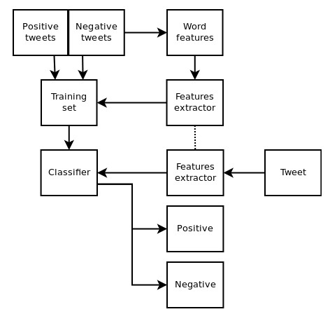
We extract two types of features from our dataset, namely unigrams and bigrams. We create a frequency distribution of the unigrams and bigrams present in the dataset and choose top N unigrams and bigrams for our analysis.
Unigrams
Probably the simplest and the most commonly used features for text classification is the presence of single words or tokens in the the text. We extract single words from the training dataset and create a frequency distribution of these words.
Bigrams
Bigrams are word pairs in the dataset which occur in succession in the corpus. These features are a good way to model negation in natural language like in the phrase – This is not good.
CLASSIFIERS
Naive Bayes
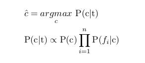
Naive Bayes is a simple model which can be used for text classification. In this model, the class ĉ is assigned to a tweet t, where
In the formula above, f i represents the i-th feature of total n features. P(c) and P(f i |c) can be obtained through maximum likelihood estimates.
Maximum Entropy
Maximum Entropy Classifier model is based on the Principle of Maximum Entropy. The main idea behind it is to choose the most uniform probabilistic model that maximizes the entropy, with given constraints. Unlike Naive Bayes, it does not assume that features are conditionally independent of each other. So, we can add features like bigrams without worrying about feature overlap. In a binary classification problem like the one we are addressing, it is the same as using Logistic Regression to find a distribution over the classes. The model is represented by
Here, c is the class, d is the tweet and λ is the weight vector. The weight vector is found by
numerical optimization of the lambdas so as to maximize the conditional probability.
Decision Tree
Decision trees are a classifier model in which each node of the tree represents a test on the attribute of the data set, and its children represent the outcomes. The leaf nodes represents the final classes of the data points. It is a supervised classifier model which uses data with known labels to form the decision tree and then the model is applied on the test data. For each node in the tree the best test condition or decision has P to be taken. We use the GINI factor to decide the best split. For a given node t, where p(j|t) is the relative frequency of class j at node t.
Random Forest
Random Forest is an ensemble learning algorithm for classification and regression. Random Forest generates a multitude of decision trees classifies based on the aggregated decision of those trees. For a set of tweets x 1 , x 2 , . . . x n and their respective sentiment labels y 1 , y 2 , . . . n bagging repeatedly selects a random sample (X b , Y b ) with replacement. Each classification tree f b is trained using a different random sample (X b , Y b ) where b ranges from 1 . . . B. Finally, a majority vote is taken of predictions of these B trees.
XGBoost
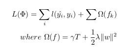
Xgboost is a form of gradient boosting algorithm which produces a prediction model that is an ensemble of weak prediction decision trees. We use the ensemble of K models by adding their outputs in the following manner
where F is the space of trees, x i is the input and y ˆ i is the final output. We attempt to minimize
the following loss function
SVM
SVM, also known as support vector machines, is a non-probabilistic binary linear classifier. For a training set of points (x i , y i ) where x is the feature vector and y is the class, we want to find the maximum-margin hyperplane that divides the points with y i = 1 and y i = −1.
The equation of the hyperplane is as follow
w . x – b = 0
We want to maximize the margin, denoted by γ, as follows:
Neural Networks
MLP or Multilayer perceptron is a class of feed-forward neural networks, which has atleast three layers of neurons. Each neuron uses a non-linear activation function, and learns with supervision using backpropagation algorithm. It performs well in complex classification problems such as sentiment analysis by learning non-linear models.
EXPERIMENTS
We perform experiments using various different classifiers. Unless otherwise specified, we use 10% of the training dataset for validation of our models to check against overfitting i.e. we use 720000 tweets for training and 80000 tweets for validation. For Naive Bayes, Maximum Entropy,Decision Tree, Random Forest, XGBoost, SVM and Multi-Layer Perceptron we use sparse vector representation of tweets. For Recurrent Neural Networks and Convolutional Neural Networks we use the dense vector representation.
Baseline
For a baseline, we use a simple positive and negative word counting method to assign sentiment to a given tweet. We use the https://www.cs.uic.edu/~liub/FBS/opinion-lexicon-English.rar of positive and negative words to classify tweets. In cases when the number of positive and negative words are equal, we assign positive sentiment. Using this baseline model, we achieve a classification accuracy of 63.48% on Kaggle public leaderboard.
Naive Bayes
We used MultinomialNB from sklearn.naive_bayes package of scikit-learn for Naive Bayes classification. We used Laplace smoothed version of Naive Bayes with the smoothing parameter α set to its default value of 1. We used sparse vector representation for classification and ran experiments using both presence and frequency feature types. We found that presence features outperform frequency features because Naive Bayes is essentially built to work better on integer features rather than floats. We also observed that addition of bigram features improves the accuracy. We obtain a best validation accuracy of 79.68% using Naive Bayes with presence of unigrams and bigrams. A comparison of accuracies obtained on the validation set using different features is shown in table 5.
Decision Tree
We use the DecisionTreeClassifier from sklearn.tree package provided by scikit-learn to build our model. GINI is used to evaluate the split at every node and the best split is chosen always. The model performed slightly better using the presence feature compared to frequency. Also using unigrams with or without bigrams didn’t make any significant improvements. The best accuracy achieved using decision trees was 68.1%. A comparison of accuracies obtained on the validation set using different features is shown in table 5.
Random Forest
We implemented random forest algorithm by using RandomForestClassifier from sklearn.ensemble provided by scikit-learn. We experimented using 10 estimators (trees) using both presence and frequency features. presence features performed better than frequency though the improvement was not substantial. A comparison of accuracies obtained on the validation set using different features is shown in table 5.
SVM
We utilise the SVM classifier available in sklearn. We set the C term to be 0.1. C term is the penalty parameter of the error term. In other words, this influences the misclassification on the objective function. We run SVM with both Unigram as well Unigram + Bigram. We also run the configurations with frequency and presence. The best result was 81.55 which came the configuration of frequency and Unigram + Bigram.
Neural Networks
We used keras with TensorFlow backend to implement the Multi-Layer Perceptron model. We used a 1-hidden layer neural network with 500 hidden units. The output from the neural network is a single value which we pass through the sigmoid non-linearity to squish it in the range [0, 1]. The sigmoid function is defined by the output from the neural network gives the probability Pr(positive|tweet) i.e. the probability of the tweets sentiment being positive. At the prediction step, we round off the probability values to convert them to class labels 0 (negative) and 1 (positive). The architecture of the model is shown in figure . Red hidden layers represent layers with sigmoid non-linearity. We trained our model using binary cross entropy loss with the weight update scheme being the one defined by Adam et. al. We also conducted experiments using SGD + Momentum weight updates and found out that it takes too long to converge. We ran our model upto 20 epochs after which it began to over fit. We used sparse vector representation of tweets for training. We found that the presence of bigrams features significantly improved the accuracy.
RESULT
By applying various algorithms the polarity of various tweets has been checked and the sentimental analysis done.
DEMO VIDEO


Reviews
There are no reviews yet.